EVALUATION OF PREDICTIVE ABILITY OF TWO ARTIFICIAL NEURAL NETWORK ALGORITHMS AND MULTIPLE REGRESSION MODEL FOR MEAT QUALITY TRAITS AFFECTED BY PRE-SLAUGHTER FACTORS
G. Ser1*, C. T. Bati2, E. Arık3 and S. Karaca1
1Department of Animal Science, Faculty of Agriculture, Van Yuzuncu Yil University, Van, Turkey
2 Department of Animal Science, Graduate School of Natural and Applied Sciences, Van Yuzuncu Yil University, Van, Turkey
3 Department of Animal Science, Graduate School of Natural and Applied Sciences, Ankara University, Ankara, Turkey
*Corresponding author’s email: gazelser@gmail.com
ABSTRACT
Recently, Artificial Neural Network (ANN) has been developed as an alternative to classical statistical methods in animal production. The methods can do classification or prediction by analyzing the information in the data set with the help of the neural network without requiring any preconditions (for example, distribution of data, non-linear data, highly correlated variables, etc.). In this context, we hypothesized that ANN, which is not only used in large and complex data sets but also estimates better in small data sets compared to classical statistical methods. The ability of ANN of Bayesian Regularization (BR-ANN) or Levenberg-Marquardt (LM-ANN) algorithms and Multiple Regression (MR) model to predict meat quality traits were assessed in a comparative study. The multilayer ANN algorithms obtained prediction data of meat quality measurements from pre-slaughter information using 1, 2, 4, 6 and 8 neurons in the hidden layer applied 10 times for each model. The performance of the methods was assessed according to the coefficient of determination (R2) criteria, root mean squared error (RMSE) and residual prediction deviation (RPD). The comparison of the findings of BR-ANN and ML-ANN algorithms showed a similar ability to predict meat quality traits (error of prediction and R2 values between 0.32-2.72 and 0.19-0.49, respectively). However, MR model predictions had lower performance than ANN algorithms, resulting in a wider error of prediction interval (0.4-3.44) and low R2 (0.16-0.44). The RPD for meat quality traits was fair for BR-ANN and LM-ANN but was poor for MR. Based on our results, the ANN algorithms produced more reasonable prediction values than the MR model. ANN algorithms can be used as an acceptable alternative method for simple physical measurements of meat quality. ANN algorithms can be used reliably in small data sets.
Key words: Bayesian networks, cattle, meat science
https://doi.org/10.36899/JAPS.2021.6.0362
Published online March 31, 2021
INTRODUCTION
Artificial Neural Network (ANN) is a tool that provides mathematical solutions to non-linear relationships or highly correlated variables in large data sets with complex structures (Prevolnik et al., 2011). There are many advantages of ANN-based methods compared to classic statistical methods (linear regression methods, growth models, partial least squares, logistic regression models, etc.). Classic statistical methods require assumptions about the distribution of variables and the structure of variables that are to be included in the model, while ANN does not require any information or preconditions about data structure. Multiple regressions are based on linear relationships between variables, but ANN has the ability to determine non-linear relationships between predicted and actual variables due to its complex functional structure (Kaewtapee et al., 2011; Okut et al., 2014). ANN is also used in the area of livestock production, as in many other areas. In the last decade, ANN was used in estimating breeding values of some traits such as milk production (Sharma et al., 2007; Shahinfar et al., 2012; Hamidi et al., 2017), reproduction (Deb et al., 2015), behavior (Tracey et al., 2011; Valletta et al., 2017), meat production and quality (Prevolnik et al., 2011), as well as in genome-enabled prediction (Okut et al., 2014; Silva et al., 2014). In meat science and technology, ANN applications are new technologies to be used in which large amounts of data with complex information (e.g., spectrometric methods, computer vision, ultrasonography techniques, etc.) are obtained (Prevolnik et al., 2011). In most of these studies, ANN methods were compared with Partial Least Squares (PLS) (Li et al., 1999; Prevolnik et al., 2009; Panagou et al., 2011). There are studies comparing some ANN models and Multiple Regression (MR) method using data obtained in the animal production field, however, the aims in these studies are generally to compare performances predictions (Norouzian and Alavijeh, 2016; Hamidi et al., 2017). Few studies have been reported regarding to ANN application to evaluate meat quality characteristics using physically measured meat traits (Santé et al., 1996; Prevolnik et al., 2009). Meat quality is determined by many pre- and post-slaughter factors that are important for breeders, the meat industry and the consumers. Meat color, fat content, sensory properties and nutrient contents are important for consumers, while water holding capacity and shelf-life are more important for the meat industry. Therefore, inspection of meat quality with novel technologies (computer vision, ultrasound, bio-sensing technologies, etc.) and also the prediction of the pre- and post-slaughter factors on meat quality accurately are very important in controlling the effects on these factors. ANN was used for the assessment of classification of carcasses and meat properties based on digital images of the meat surface or near infrared spectra mass spectroscopy hyperspectral imaging ultrasonography. Only a few studies are based on applications of ANN for meat quality assessment using several simple physical measurements of meat quality traits (Prevolnik et al., 2011). Moreover, to the best of our knowledge, the studies regarding to application of ANN to predict meat quality traits linked to pre-slaughter stress factors are limited. Therefore, the main objective of this study was to compare the prediction performances of the Artificial Neural Network algorithms of Bayesian Regularization (BR-ANN) and Levenberg-Marquardt (LM-ANN) methods and the Multiple Regression (MR) model for a data set comprising some meat quality traits linked to pre-slaughter stress.
MATERIALS AND METHODS
Animal data collection: Data of a total of 179 head of Brown Swiss (BSC) crosses and Simmental (SC) crosses with native breeds (East Anatolian Red and Native Black Bulls) and Angus (A) bulls slaughtered between 08:00-17:00 on Tuesdays and Thursdays in April, 2013 in a commercial abattoir in Van, Turkey, were used. The animals were not given any feed or water in during the lairage and, then were slaughtered without stunning. Categorical independent variables included breed (Brown Swiss, Simmental, Angus), age (< 30 months, ≥ 30 months), transport distance (<125 km, =300 km), fasting duration (1-12 hours, 13-26 hours), lairage duration (1-5 hours, 6-12 hours) and waiting type (free, tied) which were used to assess pre-slaughter stress factors. For the meat quality characteristics determination, 2.5 cm thick samples were taken from the left half of the carcasses (m.longissimus thoracis (LT); between the 11th -12th ribs) chilled for 24 hours in the cold storage depot after slaughter. Within two hours of the sampling process, water holding capacity tests were performed. After the analysis was completed, samples were preserved until the 72nd hour in high oxygen permeable PVC film at +4 °C. Following meat pH (pH72) and color (L72 and a72) measurements performed at 72nd hour, samples were placed in vacuum bags and stored at -18 °C for one month until texture analysis (Warner-Blatzer Shear Force test; WBSF). The meat pH was measured in the 12-13th ribs on the left half LT using a digital meat pH meter (Hanna HI 99163N, Hanna instruments, Romania), equipped with a penetrating electrode that was inserted to a depth of about 3 cm in the muscle. The filter paper press method described by Wierbicki and Deatherage (1958) was used to determine water-holding capacity (WHC). In order to determine meat color, a Lovibond RT-300 portable spectrophotometer (Tintometer Limited, UK) was used with daylight (D65) lighting and view system with light distribution d/8 and standard observation angle of 10° (CIELAB-illuminant D65/10°). The measurements were performed on a surface of 2.5 cm thick LT (11th–12th ribs). L*(luminosity) and a*(redness) were measured in 3 fat-free areas on the surface of each sample, and the average measurements were calculated and recorded. Texture analyses were performed according to methods described by Arık and Karaca (2017). Statistical analysis: Five different data sets were used for prediction of pH72, L72, a72, WHC and WBSF output variables by breed, age, transport distance, fasting duration, lairage duration and waiting type input variables. The data set was divided randomly as 60% training and 40% testing for the ANN performance. The artificial neural network architectures used for each dependent variable are given in Figure 1. Each architecture has a neuron in the output layer.
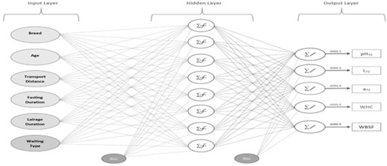
Figure 1. Multi-layer artificial neural network architectures used in the study with eight neurons in the hidden layer
In Figure 1, ANN-1,2,3,4 and 5 are artificial neural network architectures used to estimate pH72, L72, a72, WHC and WBSF, respectively. The number of hidden layers in the multilayer artificial neural was 1 and the number of neurons considered in this hidden layer were set to 1, 2, 4, 6 and 8, respectively. There was a neuron in the hidden layer of the linear neural network architecture. Linear activation function was used in both the hidden and output layer of this architecture (Figure 2). However, Tanh sigmoid was taken as the hidden layer transfer function of other neural networks. In addition, 1000 was taken as the maximum number of epochs to train in all neural networks. In order to o eliminate spurious effects caused by the starting values 10 independent LM-ANN and BR-ANN were trained for each architecture. Some elements and the information of ANN algorithms used in the selection of the best architecture are presented in Table 1.

Figure 2. Linear artificial neural network architecture
Table 1. Architecture, specification and statistical information of the ANN model
|
Elements of Architecture
|
ANN
|
|
Training algorithms
|
Bayesian Regularization and Levengberg Marquardt
|
|
Number of layers
|
3
|
|
Maximum number of epochs to train
|
1000
|
|
Learning rate
|
0.01
|
|
Hidden layer transfer function
|
Purlin* and Tanh Sigmoid
|
|
Output layer transfer function
|
Purlin
|
|
Convergence criterion
|
|
The number of variables in the input layer
|
6
|
|
Number of neurons in the output layer
|
1
|
|
Number of neurons in the hidden layer
|
1*
|
2
|
4
|
6
|
8
|
|
Estimated number of parameters
|
9*
|
17
|
33
|
49
|
65
|
*: For linear ANN networks.
Stepwise multiple regression analysis used in the study ensures the possibility of predictions by modeling the correlation between a dependent and more than one independent variable. The multiple regression models used in our study are given below (Eq. (1)):
 (1) (1)

The quality of BR-ANN, LM-ANN and MR models was evaluated using different statistical measurements: R2 (coefficient of determination) and RMSE (root mean squared error) used to evaluate between predicted and actual of meat quality traits. Also, as a measurement of quality of model RPD (residual prediction deviation), obtained by dividing the standard deviation of the observed values by the root mean square error of prediction, was assessed in Viscarra Rossel et al. (2006). Viscarra Rossel et al. (2006) categorized the RPD values into six classes: excellent (RPD>2.5), very good (RPD=2.0-2.5), good (RPD=1.8-2.0), fair (RPD=1.4-1.8), poor (RPD=1.0-1.4) and very poor model (RPD<1.0). In the presents study, the classification of Viscarra Rossel et al. (2006) for the accuracy of the prediction model was considered. According to these criteria, high R2 and RPD and low RMSE values indicate the prediction ability of the models. MATLAB R2014a (MathWorks, 2014) and R 3.5.1 (The mosaic package: Pruim et al. 2017; The psych package: Revelle, 2018; R Core Team, 2018) programs were used to create mathematical codes to develop and evaluate the ANN algorithms and MR models.
RESULTS AND DISCUSSION
Descriptive statistics for the meat quality traits are presented in Figure 3. There are missing observations for WHC and WBSF variables (n=177 and n=145, respectively).
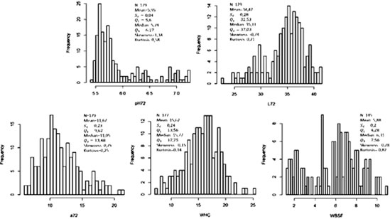
Figure 3. Descriptive statistics for meat quality traits
The results presented in Table 2 from LM-ANN and BR-ANN with different number of neurons in the hidden layer were used to evaluate the performances of two different algorithms tested in this study. R2 and RMSE criteria were considered to determine the predictive ability of the architectures in BR and LM algorithms. In both ANN algorithms, the architectures with 6 and 8 neurons in the hidden layer for the pH72 and L72 variables outperformed the other architectures. For the other traits, however, architectures with 8 neurons in hidden layer had better performance in prediction. Like many other nonlinear approaches using for the prediction purposes in the supervised machine learning, ANNs can suffer from either underfitting or overfitting. In most cases, the overfitting is more serious problem as easily led to predictions that are far beyond the range of the training data (Okut, 2016). If the number of neurons in the hidden layer are smaller than expected then underfitting may occur, while if there are too many neurons in the hidden layer then architecture can suffer from the overfitting problem. When an architecture is created for any type of training algorithms, the number of neurons may be determined based on the nature characteristic of the problem. For more complex and complicated problems, more neurons may be required. However, increasing the number of neurons in the hidden layer may lead some computation problems. Therefore, determine for the optimal number of neurons in the hidden layer for the prediction networks is an important step for ANN architectures. ANN with a smaller number of neurons may fails to capture the complex patterns between predictor variables (input) and response variable (target) in supervised learning. In contrast, ANN with excess number of neurons in hidden layer will be ended up with over-parameterization indicating over-fitting and poor generalization ability for the data. In most cases ANN with a smaller number of neurons may enable to capture the complex patterns between predictor and outcome variables (Okut, 2016). As a result, algorithms solving problems with less neurons in hidden layer can overcome with complex models as suggested in many studies (MacKay, 2008; Okut et al., 2014, Okut, 2016). However, there is no definite information about parameters like the number of neurons and number of layers that should be used in the architecture of a problem. Another approach for determining the number of neurons in the hidden layer is that the number of neurons in the hidden layer “should be between the size of the input layer and the size of the output layer or should be less than two times the input layer” (Heaton, 2017). Moharrery and Kargar (2007) pointed out that obtaining accurate estimates in ANN depends on the quality of the training data set. In general, there was lower ability to predict meat quality traits on the basis of BR-ANN and LM-ANN algorithms. Additionally, according to Haykin (2009), the number of neurons should be between 2 and 15 in order to avoid overfitting in only one hidden layer. In addition, Okut (2016) suggested that ANN architectures with certain number of neurons in the hidden layer should run, and then the predictive ability of the architecture and training algorithms should be evaluated after each obtained result for all runs. In the present study, the number of neurons were limited between 2 and 8 for nonlinear BR-ANN and LM-ANN algorithms and no over-fitting has been experienced. The Bayesian Regularization and cross-validated early stopping are two popular methods to avoid overfitting. To avoid overfitting in the Levenberg-Marquardt algorithm the early stopping rule is used. Early stopping ensures the network training is ended when the validation error is increased by 6 times the default, checking network training to prevent overtraining (Prechelt, 1997). During the training process, the errors in training and validation were monitored. When the error in the validation set increases, the training should be stopped because the point of best generalization has been reached. As a result, the Levenberg-Marquardt algorithm generally ends network training with fewer iterations compared to the Bayesian Regularization algorithm (Mohd-Safar et al., 2018; Demirezen and Fung, 2019). Therefore, if the data set to be analyzed is large, LM-ANN is a more appropriate and faster approach than BR-ANN with a successful data preprocessing stage (Demirezen and Fung, 2019). BR-ANN uses object function to avoid overfitting and improve generalization regularization technique to reach optimal level (Okut, 2016; Mohd-Safar et al., 2018). In addition, one of the information provided by the Bayesian Regularization algorithm to the user is the sufficient number of parameters in the architecture. Some parameters in this algorithm are held around zero (shrinkage) to obtain the effective number of parameters (Okut, 2016). Excessive numbers of parameters included in an architecture can be reduced to fewer numbers with this algorithm. For example, in the 8-neuron network architecture of the ph72 variable, a total of 65 parameters to be calculated, including 48 weights between each of the 6 independent variables in the input layer and 8 neurons in the hidden layer, 8 bias values added to each neuron in the hidden layer, 8 weights between the hidden layer and the output layer, and a weight in the output layer (6x8 + 8 + 8 + 1). With this algorithm, it was found sufficient to estimate 29 parameters by keeping some parameters around zero (Table 2). Thus, many parameters in this architecture have been reduced to fewer numbers.
Table 2. Results for determining the best architecture of ANN algorithms
|
Variables
|
NN
|
Bayesian Regularization
|
Levenberg-Marquardt
|
|
NE
|
RMSE
|
SNP
|
R2
(Training)
|
R2
(Test)
|
NE
|
RMSE
|
R2
(Training)
|
R2
(Test)
|
|
pH72
|
2
|
73
|
0.36
|
14
|
0.46
|
0.31
|
6
|
0.32
|
0.52
|
0.41
|
|
4
|
118
|
0.32
|
24
|
0.56
|
0.36
|
10
|
0.28
|
0.66
|
0.41
|
|
6
|
255
|
0.32
|
29
|
0.59
|
0.49
|
7
|
0.28
|
0.59
|
0.41
|
|
8
|
294
|
0.32
|
29
|
0.61
|
0.44
|
7
|
0.30
|
0.58
|
0.42
|
|
L72
|
2
|
99
|
3.06
|
12
|
0.35
|
0.15
|
6
|
2.76
|
0.41
|
0.29
|
|
4
|
186
|
2.75
|
22
|
0.48
|
0.23
|
7
|
2.88
|
0.36
|
0.29
|
|
6
|
169
|
2.76
|
23
|
0.46
|
0.27
|
6
|
2.72
|
0.42
|
0.31
|
|
8
|
234
|
2.70
|
24
|
0.48
|
0.34
|
7
|
2.60
|
0.41
|
0.30
|
|
a72
|
2
|
80
|
2.19
|
11
|
0.50
|
0.36
|
8
|
2.12
|
0.53
|
0.35
|
|
4
|
151
|
2.11
|
17
|
0.55
|
0.42
|
9
|
2.11
|
0.53
|
0.36
|
|
6
|
243
|
2.14
|
15
|
0.53
|
0.44
|
7
|
2.12
|
0.52
|
0.42
|
|
8
|
158
|
1.85
|
16
|
0.53
|
0.50
|
6
|
1.86
|
0.58
|
0.49
|
|
WHC
|
2
|
100
|
2.59
|
13
|
0.35
|
0.21
|
7
|
2.91
|
0.24
|
0.10
|
|
4
|
116
|
2.57
|
18
|
0.37
|
0.23
|
7
|
2.83
|
0.19
|
0.14
|
|
6
|
170
|
2.58
|
17
|
0.35
|
0.28
|
7
|
2.39
|
0.38
|
0.26
|
|
8
|
139
|
2.58
|
17
|
0.35
|
0.29
|
7
|
2.29
|
0.41
|
0.33
|
|
WBSF
|
2
|
193
|
2.07
|
11
|
0.28
|
0.13
|
7
|
1.98
|
0.28
|
0.21
|
|
4
|
519
|
2.22
|
6
|
0.18
|
0.10
|
9
|
1.83
|
0.37
|
0.23
|
|
6
|
739
|
2.23
|
6
|
0.19
|
0.09
|
7
|
1.88
|
0.29
|
0.21
|
|
8
|
905
|
2.21
|
6
|
0.20
|
0.19
|
6
|
1.66
|
0.37
|
0.26
|
NN: number of neurons, NE: number of epochs or iteration, RMSE: root mean squares error, SNP: sufficient number of parameters, R2: coefficient of determination, WHC: water-holding capacity (%), WBSF: warner-blatzer shear force.
The results obtained from the linear BR and linear LM-ANN algorithms are presented in Table 3 and these results are compared with MR in Table 4. According to the linear ANN results, very low estimation results were obtained from all five neural networks. However, it was seen that the linear LM-ANN architecture is better than MR for only L72 variable, and MR is better than linear neural networks for other variables.
Table 3. Results of linear neural networks
|
Variables
|
Bayesian Regularization
|
Levenberg-Marquardt
|
|
NE
|
RMSE
|
SNP
|
R2
(Training)
|
R2
(Test)
|
NE
|
RMSE
|
R2
(Training)
|
R2
(Test)
|
|
pH72
|
1000
|
0.41
|
7
|
0.33
|
0.20
|
6
|
0.40
|
0.31
|
0.18
|
|
L72
|
1000
|
3.40
|
7
|
0.20
|
0.15
|
6
|
3.39
|
0.24
|
0.23
|
|
a72
|
1000
|
2.36
|
7
|
0.44
|
0.36
|
6
|
2.34
|
0.43
|
0.36
|
|
WHC
|
1000
|
2.87
|
6
|
0.20
|
0.13
|
6
|
2.80
|
0.20
|
0.15
|
|
WBSF
|
1000
|
2.32
|
6
|
0.16
|
0.11
|
6
|
2.17
|
0.17
|
0.12
|
NE: number of epochs or iteration, RMSE: root mean squares error, SNP: sufficient number of parameters, R2: coefficient of determination, WHC: water-holding capacity (%), WBSF: warner-blatzer shear force.
Table 4. Comparison results for linear ANN algorithms and MR model for meat quality traits
|
Variables
|
Bayesian Regularization
|
Levenberg-Marquardt
|
Multiple Regression
|
|
RMSE
|
R2
|
RPD
|
RMSE
|
R2
|
RPD
|
RMSE
|
R2
|
RPD
|
|
pH72
|
0.41
|
0.20
|
1.20
|
0.40
|
0.18
|
1.18
|
0.40
|
0.33
|
1.25
|
|
L72
|
3.40
|
0.15
|
1.10
|
3.39
|
0.23
|
1.19
|
3.44
|
0.17
|
1.13
|
|
a72
|
2.36
|
0.36
|
1.32
|
2.34
|
0.36
|
1.32
|
2.35
|
0.44
|
1.36
|
|
WHC
|
2.87
|
0.13
|
1.11
|
2.80
|
0.15
|
1.12
|
2.93
|
0.17
|
1.13
|
|
WBSF
|
2.32
|
0.11
|
1.03
|
2.17
|
0.12
|
1.03
|
2.26
|
0.16
|
1.05
|
RMSE: root mean squares error, R2: coefficient of determination, RPD: residual prediction deviation, WHC: water-holding capacity (%), WBSF: warner-blatzer shear force.The results obtained for the best architectures from the BR and LM-ANN algorithms and stepwise MR are presented in Table 5. The pH72, L72, and a72 prediction values obtained with the both ANN algorithms were considerably better compared to those for MR. The RMSE and R2 for pH72, L72 and a72 were within the range of 0.32–3.44 and 0.17%-0.50%, respectively. On the other hand, the WHC and WBSF variables had lower prediction performance for three algorithms, but it appeared the BR-ANN algorithm especially had much lower R2 and higher prediction of error values compared to LM-ANN. It is interesting to observe that the LM-ANN algorithm is more successful than BR-ANN and MR in estimating the missing observations (34 missing observations, nearly 19%) determined in the WBSF variable.
In present study, BR-ANN and LM-ANN algorithms provided the largest RPD values for pH72 and a72 predictions. However, for the L72, WHC and WBSF variables, the smallest RPD values were obtained with three methods. While BR-ANN and LM-ANN algorithms were considered to be fair for the prediction of the pH72 and a72 variables according to the classification of Viscarra Rossel et al. (2006), three methods were poor for the prediction of L72, WHC and WBSF. But, for the WBSF variable, the LM-ANN algorithm interestingly estimated an RPD value (1.30) greater than for WHC and L72 and the means square error was smaller (2.74). Nevertheless, when three algorithms were evaluated, they provided smaller RPD values than expected. According to Prevolnik et al. (2009), other factors such as measurement location, sampling site and other uncontrolled environmental factors contributing to uncertainty should be considered as well as the high predicted errors with the smallest RPD values. In addition to these effects, we speculate the number of missing observations, non-linear relationships or variations among measured values could cause lower RPDs.
Table 5. Results of comparison for the ANN algorithms and MR model for meat quality traits
|
Variables
|
Bayesian Regularization
|
Levenberg-Marquardt
|
Multiple Regression
|
|
RMSE
|
R2
|
RPD
|
RMSE
|
R2
|
RPD
|
RMSE
|
R2
|
RPD
|
|
pH72
|
0.32
|
0.49
|
1.51
|
0.44
|
0.42
|
1.48
|
0.40
|
0.33
|
1.25
|
|
L72
|
2.70
|
0.34
|
1.34
|
2.72
|
0.31
|
1.23
|
3.44
|
0.17
|
1.13
|
|
a72
|
1.85
|
0.50
|
1.44
|
1.86
|
0.49
|
1.41
|
2.35
|
0.44
|
1.36
|
|
WHC
|
2.58
|
0.29
|
1.24
|
2.29
|
0.33
|
1.26
|
2.93
|
0.17
|
1.13
|
|
WBSF
|
2.20
|
0.19
|
1.09
|
1.66
|
0.26
|
1.30
|
2.26
|
0.16
|
1.05
|
RMSE: root mean squares error, R2: coefficient of determination, RPD: residual prediction deviation WHC: water-holding capacity (%), WBSF: warner-blatzer shear force.The variable pH72, which has the smallest error between the actual and predicted values in three models, is represented in Fig. 4. If the prediction curve of a method follows the true value curve it is assessed as successful, whereas differentiation in the curve is an indicator of prediction error. As seen in Fig. 4, the BR-ANN algorithm appears to provide the best fit curve.
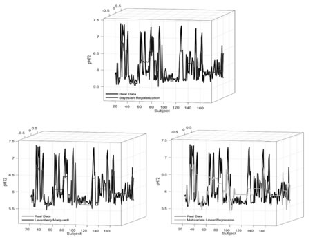
Figure 4. Prediction performance for the pH72 variableThe prediction error of the prediction values for only the pH72 variable with three methods shows Fig. 5. Accordingly, the prediction error fluctuation was in the order of MR, LM-ANN and BR-ANN.
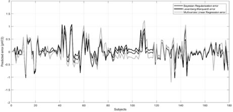
Figure 5. Prediction errors for the pH72 variable
Conclusion: Findings in the present study demonstrate that ANN algorithms promised better prediction ability than the MR model for the basis of simple meat quality traits like Both algorithms of ANN have the ability to predict simple physical quality traits of meat, decrease in errors and better prediction compared to MR. However, the multilayer artificial neural networks algorithms, neuron numbers, determination of activation function and epoch selections are important in obtaining valid predictions. The MR method does not have this flexible adjustment feature compared to ANN. The method is more conservative than ANN. We propose that ANN algorithms should be preferred over more traditional methods, especially in small data sets in animal sciences.
Ethical statement: Permission for Animal research procedures was granted by the Local Animal Ethics Committee of Yuzuncu Yil University in Van, Turkey (Decision No. 2013/06).
Competing interests: The authors declare that they have no conflict of interest.
REFERENCES
- Arik, E.and S. Karaca (2017). The effect of some pre-slaughter factors on meat quality of bulls slaughtered in a commercial abattoir in Turkey. Indian J. Anim. Res. 51:557-563. DOI: 10.18806/ijar.v0iOF.4563
- Deb, R., U. Singh, T.V. Raja, S. Kumar, S. Tyagi, R.R. Alyethodi, R. Alex, G. Sengar and S. Sharma (2015). Designing of an artificial neural network model to evaluate the association of three combined Y-specific microsatellite loci on the actual and predicted postthaw motility in crossbred bull semen. 83:1445-50. DOI: 10.1016/j.theriogenology.2015.01.014
- Hamidi, S.P., M.R. Mohammadabadi, M.A. Foozi and H. Nezamabadi-Pour (2017). Prediction of breeding values for the milk production trait in Iranian Holstein cows applying artificial neural networks. Lives. Sci. Tech. 5:53-61. DOI: 10.22103/jlst.2017.10043.1188
- Haykin, S (2009). Neural Networks and Learning Machines, Third Edition, Pearson Educaion, New Jersey.
- Kaewtapee, C., C. Khetchaturat and C. Bunchasak (2011). Comparison of growth models between artificial neural networks and nonlinear regression analysis in Cherry Valley ducks. Appl. Poult. Res. 20: 421-428.
- Li, J., J. Tan, F.A. Martz and H. Heymann (1999). Image texture features as indicators of beef tenderness, Sci. 53:17-22. DOI: 10.1016/S0309-1740(99)00031-5
- MacKay, J. C. D. (2008). Information Theory, Inference and Learning Algorithms. Cambridge University Press, Cambridge-UK.
- (2014). MATLAB and Statistics Toolbox Release 2014a, The MathWorks, Inc., Natick, Massachusetts, USA.
- Moharrery, A., A. Kargar (2007). Artificial Neural Network for prediction of plasma hormones, liver enzymes and performance in broilers. Anim. Feed Sci. 16:293-304. DOI: 10.22358/jafs/66751/2007
- Mohd-Safar, N.Z., D. Ndzi, I. Kagalidis, Y. Yang, A. Zakaria (2018). Short-Term Localized Weather Forecasting by Using Different Artificial Neural Network Algorithm in Tropical Climate. In: Bi Y., Kapoor S., Bhatia R. (eds) Proceedings of SAI Intelligent Systems Conference (IntelliSys) 2016. Lecture Notes in Networks and Systems, vol 16. Springer, Cham.
- Norouzian, M.A., M.V. Alavijeh (2016). Comparison of Artificial Neural Network and Multiple Regression Analysis for Prediction of Fat Tail Weight of Sheep. Iranian J. Appl. Anim. Sci. 6: 895-900.
- Okut, H., X.L. Wu, G.J. Rosa, S. Bauck, B.W. Woodward, R.D. Schnabel, J.F. Taylor, D. Gianola (2014). Predicting expected progeny difference for marbling score in Angus cattle using artificial neural networks and Bayesian regression models. Sel. Evol. 45:34. DOI: 10.1186/1297-9686-45-34
- Okut, H. (2016). Bayesian regularized neural networks for small n big p data. In Artificial Neural Networks-Models and Applications; IN-TECH: Munich, Germany.
- Panagou, E.Z., F.R. Mohareb, A.A. Argyri, C.M. Bessant, G.J.E. Nychas (2011). A comparison of artificial neural networks and partial least squares modelling for the rapid detection of the microbial spoilage of beef fillets based on Fourier transform infrared spectral fingerprints. Food Microbiol. 28:782-790. DOI: 1016/j.fm.2010.05.014
- Prechelt, L. (1997). Automatic Early Stopping Using Cross Validation: Quantifying the Criteria. Appeared in Neural Networks. University Karlsruhe D-76128. Karlsruhe. Germany.
- Prevolnik, M., D. Skorjanc, M. Candek-Potokar, M. Novic (2011). Application of artificial neural networks in meat production and technology, In: Artificial Neural Networks Industrial and Control Engineering Applications. edited by: Suzuki, K., InTech, London, UK, 223-240.
- Prevolnik, M., M. Candek-Potokar, M. Novic, D. Skorjanc (2009). An attempt to predict pork drip loss from pH and colour measurements or near infrared spectra using artificial neural networks. Sci. 83:405-11. DOI: 10.1016/j.meatsci.2009.06.015
- 18. Pruim, R., D.T. Kaplan, and N.J. Horton (2017). The mosaic Package, Helping Students to 'Think with Data' Using R, The R Jour. 9(1): 77-102.
- R Core Team, 2018. A language and environment for statistical computing, R Foundation for Statistical Computing, Vienna, AustriA.
- 20. Revelle, W. (2018). Procedures for Personality and Psychological Research, Northwestern University, Evanston, Illinois, USA, https://CRAN.R-project.org/package=psych, Version 1.8.4.
- Santé, V.S., A. Lebert, G. Le Pottier, A. Ouali (1996). Comparison between two statistical models for prediction of turkey breast meat colour. Meat Sci. 43:283-290. DOI: 10.1016/S0309-1740(96)00026-5
- Shahinfar, S., H. Mehrabani-Yeganeh, C. Lucas, A. Kalhor, M. Kazemian, K.A. Weigel (2012). Prediction of breeding values for dairy cattle using artificial neural networks and neuro-fuzzy systems. Math. Methods. Med. 1-9. DOI: 10.1155/2012/127130
- Sharma, A.K., R.K. Sharma, H.S. Kasana (2007). Prediction of first lactation 305-day milk yield in Karan Fries dairy cattle using ANN modeling. Appl. Soft. Comput. 7:1112-1120. DOI: 1016/j.asoc.2006.07.002
- Silva, G.N., R.S. Tomaz, I.D.C. Sant'Anna, M. Nascimento, L.L. Bhering, C.D. Cruz (2014). Neural networks for predicting breeding values and genetic gains. Agr. 71:494-498. DOI: 10.1590/0103-9016-2014-0057
- Tracey, J.A., J. Zhu, K.R. Crooks (2011). Modeling and inference of animal movement using artificial neural networks. Ecol. Stat. 18:393-410. DOI: 10.1007/s10651-010-0138-8
- Valletta, J.J., C. Torney, M. Kings, A. Thornton, J. Madden (2017). Applications of machine learning in animal behaviour studies. Beh. 124:203-220. DOI: 10.1016/j.anbehav.2016.12.005
- Viscarra Rossel, R.A., R.N. McGlynn, A.B. McBratney (2006). Determining the composition of mineral-organic mixes using UV–vis–NIR diffuse reflectance spectroscopy. 137: 70-82.
- Wierbicki, E., F.E. Deatherage (1958). Determination of water-holding capacity of fresh meats. Agri. Food Chem. 6:387-392.
|