EXAMINATION OF THE RELATIONSHIP AMONG PLANT CHARACTERISTICS AFFECTING YIELD IN PEA PLANTS WITH MARS ALGORITHM
S. Celik1, A. Bakoglu2 and M. İ. Çatal3
1Department of Animal Science, Faculty of Agriculture, University of Bingol, Turkey
2Department of Plant and Animal Production, Vocational School of Pazar, University of Recep Tayyip Erdogan, Turkey.
3Department of Field Crops, Faculty of Agriculture and Natural Sciences, Recep Tayyip Erdogan University, Turkey
Corresponding author e-mail: senolcelik@bingol.edu.tr
ABSTRACT
This study was conducted to investigate the effects of some plant characteristics on green fodder and dry matter yield in pea plants. Plant characteristics; height (PH), pod number (PN), number of seeds in pods (SeedP), straw weight per plant (SeedW), straw yield (STY), seed yield (SeedY), Harvest Index (Hi) and 1000 Seed Weight (SeedWth) were evaluated for some yield traits: green fodder yield (GreHYi:), dry matter yield (DryHYi) . To estimate green fodder and dry matter yield in pea plant, two different MARS (Multivariate Adaptive Regression Splines) algorithms were performed. In both MARS models, a 2nd-degree interaction equation was obtained. To determine the suitability of the model, it has been considered that generalized cross-validation (GCV), root mean square error (RMSE), Akaike's Information Criterion (AIC) statistics to be minimum and coefficient of determination (R2) and adjusted coefficient of determination (Adj. R2) values to be maximum. In two separate MARS models formed to estimate green fodder and dry matter yield, R2 values were 0.998 and 0.998 respectively; Adj. R2 values were 0.999 and 0.998, RMSE values were 8.268 and 0.571, SDratio values were 0.037 and 0.019, and AIC values were 241 and 21. The greatest increase in green fodder yield in pea plants occurred when plant height was less than 42. The contribution of plant height to yield was 332 kg. The biggest increase in dry matter yield occurred when the harvest index was 20.5%. The contribution of harvest index to dry matter yield was 16.4. It has been noted that MARS is a good model in terms of predicting yield in pea plants.
Keywords: Pea, yield, MARS algorithm, Generalized Cross Validation (GCV)
https://doi.org/10.36899/JAPS.2021.6.0366
Published online March 31, 2021
INTRODUCTION
Pea is an important plant in human and animal nutrition because of its high protein level (23 - 33%). Pea is cultivated for many purposes. Pea grains are eaten fresh or processed as canned food. The pea grains have a high sugar rate. Dry pea grains are broken and used to make soup. On the other hand, the pea grains are used in animal feed. Pea is used for seed, hay, pasture, silage, and green manure (Erac and Ekiz, 1985). It is rich in phosphorus and calcium; and also, a good source of vitamins, especially vitamins A and D. These qualities make field peas one of the best feeds for animals and almost indispensable for efficient, economical livestock feeding (Açıkgöz, 2001, Anonymous, 2003).
In Idaho and Oregon varieties among the US varieties of feed peas, which are subjected to adaptation trials, it has been reported that yields of 119-241 kg/da, plant height of 60-75 cm, weight of 1000 seeds around 195-248 g have been obtained (Guy, 2002). In the study conducted with some feed pea routes; characters, such as morphological characters, plant height, number of main branches, number of leaflets on the leaf, stem diameter, number of seeds in pods, number of broad beans, dry matter yield, seed yield and protein ratio were different. The findings showed that the maximum dry matter yield was 731.9 kg/da and the highest seed yield was 259.0 kg/da (Tekeli and Ateş, 2003). In 2019, 146090 decares of peas (green fodder) were grown in Turkey, 283928 tons were produced and 1943.5 kg yield per decare was obtained (TSI, 2019a). In the same year, 7813 peas (dry seed) were planted and 2193 tons were produced and 281 tons of yield per decare were obtained (TSI, 2019b).
There are studies on feed pea conducted using path analysis using morphological features of the plants (Khan et al., 2017; Gautam et al., 2017). Direct and indirect effects of different traits on yield in peas were displayed using path analysis by Nawab et al. (2008), Devi et al. (2017) and Khan et al. (2017).
One of the methods to examine the relationship between plant yield and other properties utilizing morphological features of the plant is MARS (Multivariate Adaptive Regression Splines) algorithm. The MARS algorithm is a method used to investigate the effects of independent variables on the dependent variable in data analysis. MARS algorithm is a method that was developed by Friedman (1991) using complex algorithms that can evaluate multiple variables together. There have been studies conducted in the agricultural field with the MARS algorithm (Eyduran et al., 2017; Aksoy et al., 2018; Aytekin et al., 2018).
The MARS technique is a nonparametric regression technique and can be seen as an extension of linear models that automatically models nonlinearities and interactions. MARS models are more flexible than linear regression models and they are simple to understand and interpret. The MARS technique can handle both numeric and categorical data, and it tends to be better than recursive partitioning for numeric data (Bishop, 2006). To adjust ideas, building MARS models often requires little or no data preparation. The hinge functions automatically partition the input data, so the effects of outliers are included. From this point, the MARS technique is similar to recursive partitioning which also partitions the data into disjoint regions, using a different method. MARS models tend to have a good bias-variance trade-off, and they are flexible enough to model nonlinearity and variable interactions (García Nieto et al. 2011; Vidoli 2011; García Nieto et al. 2012).
Assumptions such as continuity of all variables, absence of significant outliers in the data, equality of variances, normal distribution of residual variables, and absence of significant multi-linearity between independent variables should be provided to create a multiple regression or multivariate regression model. However, the MARS model is a non-parametric method that does not require assumptions about the functional relationship between variables. The MARS method creates a flexible regression model using basic functions that correspond to different ranges of independent variables. Thus, it is an alternative method that can be used in many data sets instead of regression analysis. The present study aims to investigate the green fodder and dry matter yield estimation model using morphological features of the plant.
MATERIALS AND METHODS
This study was conducted in the Agricultural Faculty, Bingöl University (38°53´55.86´´ N, 40°29´15.07´´ E, altitude 1166 m) in Bingöl (Turkey) province, during the growing season of 2015. Soil sample was collected at a depth of 0-20 cm. The soils texture was clay loam, available P2O5 327.5 kg ha-1 and available K2O 1150 kg ha-1, quite weak in organic matter content (0.26%), pH 6.85. Average temperatures of 12.2 and 21.5°C were recorded between April and July during the growing season of 2015 and long-term averages in Bingöl, respectively. Average long-term total precipitations of 947.3 mm were recorded, 223.2 mm between April and July during the 2015 and long-term periods in Bingöl, respectively. Six pea lines (88PO38-4-3-683, SPRİNGPEA3638, P57B, P57K, P101, P104) and six genotypes (ATOS and ÖZKAYNAK) were obtained from Institute of Southeastern Agricultural research, two genotypes (ÜRÜNLÜ and GÖLYAZI) from the Agricultural Faculties of Uludag, University. “Variety’’ regard as cultivar species and “line’’ is usually a product of breeding that is not officially registered yet at a national level. Field experiments were designed according to randomized complete block design (RCBD) with three replications during 2015. Seeds were sown on the first of April, 2015 in Bingöl conditions.
Plot size was 5 x 1.8 m. Sowing rate was 120 kg ha-1. 30 N kg ha-1 and 80 P2O5 kg ha-1 were uniformly applied to the soil before sowing. In trial parcels, 50% vegetative properties in bloom and generative properties were detected in the harvest maturity period; studies were conducted with ten plants selected randomly from each parcel. In this study, several hay quality, traits such as plant height (cm), green herbage yield (green fodder yield) and dry herbage yield (dry matter yield) (kg da -1), cut yield (kg da -1), number of pod per plant, number of seed per plant, number of seed per pod, seed weight per plant (g), straw yield per plant (g), straw yield (kg da -1), seed weight (kg da -1), 1000 seed weight (%) and harvest index (%), were analyzed.
MARS technique not only examines the relationships of each independent variable with the dependent variable, but also determines the interactions among the independent variables and reveals the effects of interactions on the dependent variable (Hastie et al., 2001; Tunay, 2001).
In the MARS algorithm, assumptions are not required about functional relationships between the dependent variable and independent variables. Instead, this relation is uncovered from a set of coefficients and piecewise polynomials of degree q (basis functions) that are completely driven by the regression data (x, y). The MARS algorithm is established by fitting basis functions to distinct intervals of the independent variables (Friedman, 1991; Vidoli 2011; García Nieto et al., 2012).
The spline forming the basis for MARS is a new mathematical process in complex curve drawings and function estimates. Spline straightening method is a method enabling the control of the non-parametric error variance obtained when two or higher-grade polynomials are used (Kaki et al., 2004).
In MARS terminology, the joining points of the polynomials are called nodes. A model can be estimated with a sufficient number of nodes (Hastie et al., 2008).
The model installation takes place in two phases. Primarily, the MARS model is described one and only input variable x. Candidate knots are placed at random situations within the range of each predictor to define a pair of basic functions. At each step, the knot and its corresponding pair of basic functions are fitted to yield the maximum reduction in sum-of-squares residual error. New basic functions are added until the threshold value is achieved. The forward phase selection of the basic function causes a very complex and over-fitted model. Even if this resulted function fits the training data well, it has a low predictive capacity for the new dataset. The generalized cross-validation error is calculated in each step, which considers both the residual error and the model complexity as well. Generalized Cross Verification (GCV) was introduced by Craven and Wahba (1979) and expanded for MARS by Friedman (1991).
GCV considers both the residual error and the model complexity and GCV;

Calculated from
C=1+cd equations. In the equality,
N: shows the number of observations in the data set,
c: The c is the penalty term for adding an independent variable that does not affect the dependent,
d: is the efficient degree of freedom and the number of independent basic functions,
C: Cost-complexity of added basic functions and
B: shows the number of regression models established by MARS model.
As a result of the calculations, it was found that the value of 2 <d <3 was the best for the C value. (Briand et al., 2000).
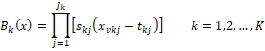
The MARS Model consists of the results of the determinants that give basic functions and model parameters (estimated by the least-squares method) data entries. General MARS model is as follows.

Here;
k: The number of nodes,
K: The number of basic functions,
X: Independent variable,
 : k. Basic function coefficient, : k. Basic function coefficient,
 : Fixed term in model : Fixed term in model
 : t. For the independent variable, k. is the basic function (Hill and Lewicki, 2006). : t. For the independent variable, k. is the basic function (Hill and Lewicki, 2006).
This function consists of the cutting parameter and the weighted sum of one or more basic functions (Oğuz, 2014).
The MARS method uses a fragmented polynomial function to determine the basic functions. Regression sections passing through the points closest to all values can be formed. Regression section functions are a continuous function that can be obtained by combining partial polynomial basic functions in nodes. The constants in the basic functions are found by the method of the smallest squares. They are described as basic functions
Here  : Interaction degree, : Interaction degree,  , ,  , ,
 : node value indicates : node value indicates  : independent variable value (Hill and Lewicki, 2006). : independent variable value (Hill and Lewicki, 2006).
The MARS model was built by the basic functions fitting of different ranges of independent variables. Polynomials, often referred to as splines, have neat pieces connected together. In MARS terminology, the joining points of the polynomials are called nodes and shown with t. MARS  and and  piecewise linear use expansions in the basic functions. The parameter is the node of the basic functions. Therefore, piecewise linear use expansions in the basic functions. The parameter is the node of the basic functions. Therefore,

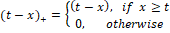
equations are used (Hastie et al., 2008).
Each function value is a piecewise linear with a node. They are linear chains. MARS creates flexible models using piecewise linear regression and uses separate regression trends in different ranges of the independent variable to eliminate non-linear states. The points where the regression slope changes and passes from one range to another is called a node (Chen and Lee, 2005).
To determine the predictive performance of the MARS algorithm, the following goodness of fit criteria were investigated (Willmott and Matsuura, 2005; Takma et al., 2012; Ali et al., 2015):
1. Coefficient of Determination: The coefficient of determination, R2, is used to analyze how differences in one variable can be explained by a difference in another variable.
 2. Adjusted Coefficient of Determination: Adjusted coefficient of determination is the adjusted value of the coefficient of determination in which the number of variables of the data set is taken into consideration. 2. Adjusted Coefficient of Determination: Adjusted coefficient of determination is the adjusted value of the coefficient of determination in which the number of variables of the data set is taken into consideration.

3. Root-mean-square error (RMSE) presented by the following formula:

The root mean square error (RMSE) has been used as a standard statistical parameter to measure model performance in several sciences. The parameter indicates the standard deviation of the residuals or how far the points are from the modelled line.
4. Standard deviation ratio (SDratio):
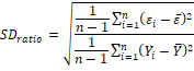
SD ratio estimates should be less than 0.40 for a good fit explained in some studies (Grzesiak et al., 2003; Grzesiak and Zaborski, 2012).
5. Akaike Information Criteria (AIC): AIC test how well model fits the data set without over-fitting it.
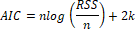
where: RSS: Residual sum square, n is the number of cases in a set, k is the number of model parameters, Yi is the observed value of an output variable, Yip is the predicted value of an output variable,  is the residual values of model, is the residual values of model,  is the average of residual values. is the average of residual values.
Statistical evaluations on the MARS algorithm were specified using the R software (R Core Team, 2018) program.
RESULTS
Descriptive statistics belong to pea are given in Table 1. Simple correlation coefficients calculated among characteristics in the pea plant are presented in Table 2. Positive significant relationships were obtained between green fodder yield and dry yield (r=0.780**), the number of pods (r=0.535**), number of seeds in pods (r=0.313*) and straw weight per plant (r=0.422**). Also, positive significant relationships were found between dry matter yield and green fodder yield (r=0.780**), number of pods (r=0.307**) and harvest index (r=0.355**).
Table 1. Descriptive statistics for pea plant
|
Character
|
Mean
|
Std. Deviation
|
N
|
|
PH
|
62.44
|
19.504
|
42
|
|
GreHYi
|
958.10
|
226.161
|
42
|
|
DryHYi
|
148.07
|
31.140
|
42
|
|
PN
|
15.33
|
7.234
|
42
|
|
SeedP
|
67.64
|
30.433
|
42
|
|
SeedW
|
8.813
|
6.317
|
42
|
|
STY
|
486.500
|
259.594
|
42
|
|
SeedY
|
184.238
|
140.759
|
42
|
|
Hi
|
27.019
|
8.461
|
42
|
|
SeedWth
|
121.491
|
17.405
|
42
|
PH: Plant height (cm), GreHYi: Green fodder yield (kg da-1), DryHYi: Dry yield (kg da-1), PN: Number of pods per plant, SeedP: Number of seeds in pods, SeedW: Straw Weight per plant, STY: Straw Yield, SeedY: Seed Yield, Hi: Harvet Index, SeedWth: 1000 Seed Weight.
Table 2. Correlation coefficients among the characteristics in pea plant (r).
|
Character
|
1
|
2
|
3
|
4
|
5
|
6
|
7
|
8
|
9
|
10
|
|
1-PH
|
1
|
0.145
|
0.272
|
0.012
|
-0.202
|
-0.098
|
0.338*
|
0.042
|
0.274
|
-0.441**
|
|
2-GreHYi
|
0.145
|
1
|
0.780**
|
0.535**
|
0.313*
|
0.422**
|
0.205
|
0.283
|
0.166
|
0.166
|
|
3-DryHYi
|
0.272
|
0.780**
|
1
|
0.307*
|
0.046
|
0.147
|
0.239
|
0.173
|
0.355*
|
0.031
|
|
4-PN
|
0.012
|
0.535**
|
0.307*
|
1
|
0.787**
|
0.756**
|
0.064
|
0.388*
|
0.061
|
0.421**
|
|
5-SeedP
|
-0.202
|
0.313*
|
0.046
|
0.787**
|
1
|
0.863**
|
0.028
|
0.426**
|
-0.049
|
0.514**
|
|
6-SeedW
|
-0.098
|
0.422**
|
0.147
|
0.756**
|
0.863**
|
1
|
0.208
|
0.604**
|
0.176
|
0.537**
|
|
7-STY
|
0.338*
|
0.205
|
0.239
|
0.064
|
0.028
|
0.208
|
1
|
0.755**
|
0.362*
|
-0.130
|
|
8-SeedY
|
0.042
|
0.283
|
0.173
|
0.388*
|
0.426**
|
0.604**
|
0.755**
|
1
|
0.376*
|
0.499**
|
|
9-Hi
|
0.274
|
0.166
|
0.355*
|
0.061
|
-0.049
|
0.176
|
0.362*
|
0.376*
|
1
|
0.080
|
|
10-SeedWth
|
-0.441**
|
0.166
|
0.031
|
0.421**
|
0.514**
|
0.537**
|
-0.130
|
0.499**
|
0.080
|
1
|
*(p<0.05), **(p<0.01), ***(p<0.001). t test was used for testing the significance of correlation.
Model 1: To estimate green fodder (GreHyi), the MARS algorithm was created by selecting the following independent variables, plant height (PH), number of pods in the plant (PN), number of seeds in pods (SeedP), seed number in the pod (SeedN), seed weight in the plant (SeedW), straw weight in plant (StW), straw yield (STY), seed yield (SeedY), 1000 seed weight (SeedWth) and harvest index (Hi). Here, dependent variable is GreHyi. The independent variables are PH, PN, SeedP, SeedN, SeedW, StW, STY, SeedY, SeedWth and Hi.
The generated algorithm was a model with 32 basic functions, including second order fixed term. For this model, it was estimated GCV=1206, R2=0.999, Adj. R2=0.995, SDratio=0.037, RMSE=8.268 and AIC=241. These results pointed out very high goodness of fit for the MARS model analyzed. To warrant the prediction ability of the MARS model, the cross-validation was used. The basic functions and coefficients, according to the model, are presented in Table 3.
Table 3. Model 1-MARS algorithm results in pea estimation of green fodder yield
Coefficients Estimate Std. Error t value Pr(>|t|)
(Intercept) 6.502e+02 1.199e+02 5.423 0.000292 ***
bx[, -1]h(PN-12) -1.246e+02 1.485e+01 -8.394 7.71e-06 ***
bx[, -1]h(12-PN) -4.774e+01 5.258e+00 -9.079 3.82e-06 ***
bx[, -1]h(StW-22.76) -3.871e+01 9.559e+00 -4.050 0.002323 **
bx[, -1]h(22.76-StW) -7.464e+01 6.812e+00 -10.956 6.84e-07 ***
bx[, -1]h(PH-42) 5.369e+00 7.006e-01 7.662 1.71e-05 ***
bx[, -1]h(42-PH) 3.320e+02 2.120e+02 15.656 2.32e-08 ***
bx[, -1]h(SeedWTh-130.3) -1.132e+01 2.735e+00 -4.140 0.002011 **
bx[, -1]h(130.3-SeedWth) 7.780e+01 3.720e+00 20.912 1.39e-09 ***
bx[, -1]h(42-PH)*Hi -1.120e+02 7.237e+00 -15.474 2.59e-08 ***
bx[, -1]h(22.76-StW)*STY -3.285e-01 1.950e-02 -16.842 1.14e-08 ***
bx[, -1]SeedN*h(StW-22.76) -1.442e+01 9.482e-01 -15.205 3.07e-08 ***
bx[, -1]SeedP*h(StW-22.76) 4.856e+00 3.044e-01 15.954 1.93e-08 ***
bx[, -1]h(22.76-StW)*STY*SeedWTh 2.205e-03 1.494e-04 14.762 4.08e-08 ***
bx[, -1]SeedN*h(130.3-SeedWTh) -7.967e+00 4.493e-01 -17.730 6.95e-09 ***
bx[, -1]SeedP*h(22.76-StW)*STY 1.651e-03 1.271e-04 12.983 1.39e-07 ***
bx[, -1]h(PH-42)*h(StW-12.22) -2.578e-01 5.060e-02 -5.094 0.000468 ***
bx[, -1]h(PH-42)*h(12.22-StW) 1.863e+00 1.706e-01 10.919 7.06e-07 ***
bx[, -1]h(42-PH)*SeedWth -3.462e+01 2.051e+00 -16.883 1.12e-08 ***
bx[, -1]h(42-PH)*SeedWth*Hi 1.184e+00 7.011e-02 16.890 1.11e-08 ***
bx[, -1]h(SeedW-6.02) -8.472e+00 2.192e+00 -3.865 0.003133 **
bx[, -1]h(6.02-SeedW) 4.355e+01 5.344e+00 8.150 1.00e-05 ***
bx[, -1]PN*SeedN*h(StW-22.76) -3.435e+00 2.758e-01 -12.456 2.06e-07 ***
bx[, -1]SeedN*h(22.76-StW) 5.339e+00 6.071e-01 8.795 5.09e-06 ***
bx[, -1]h(SeedY-150) -4.394e-01 8.537e-02 -5.147 0.000433 ***
bx[, -1]h(150-SeedY) -2.177e+00 1.773e-01 -12.276 2.36e-07 ***
bx[, -1]PH*h(130.3-SeedWth) -2.554e-01 2.973e-02 -8.591 6.27e-06 ***
bx[, -1]h(PN-13) 1.153e+02 1.474e+01 7.821 1.44e-05 ***
bx[, -1]h(12-PN)*SeedP*STY 3.381e-03 3.407e-04 9.924 1.70e-06 ***
bx[, -1]h(SeedWth-107.1) 1.159e+01 2.807e+00 4.130 0.002043 **
bx[, -1]SeedN*SeedW*h(130.3-SeedWth) 9.162e-02 2.494e-02 3.674 0.004289 **
bx[, -1]h(StW-10.33) 2.141e+01 6.750e+00 3.171 0.009966 **
The most effect results obtained in accordance with Model-1 in Table 3 are described below.
· When PH≤42, green fodder yield increases by 332 kg (the contribution of this basic function to the model is 332)
· When PN>13, green fodder yield increases by 115 kg (the contribution of this basic function to the model is 115),
· When SeedWth ≤ 130.3 g, green fodder yield increases by 77.8 kg,
· When SeedW≤6.02, green fodder yield increases by 43.6 kg,
· When StW>10.3, green fodder yield increases by 21.4 kg,
· When PN>12 and SeedWth, green fodder yield decreases by 125 kg (the contribution of this basic function to the model is -125),
· When PH≤42 and Hi, green fodder yield decreases by 112 kg,
· When StW≤22.8, green fodder yield decreases by 74.6 kg,
· When PN≤12, green fodder yield decreases by 47.7 kg,
· When StW>22.8, green fodder yield decreases by 38.7 kg,
The MARS equation of Model 1 is as follows.
GreHYi = 650
+ 332 * max(0, 42 - PH)
+ 5.37 * max(0, PH - 42)
- 47.7 * max(0, 12 - PN)
- 125 * max(0, PN - 12)
+ 115 * max(0, PN - 13)
+ 43.6 * max(0, 6.02 - SeedW)
- 8.47 * max(0, SeedW - 6.02)
+ 21.4 * max(0, StW - 10.3)
- 74.6 * max(0, 22.8 - StW)
- 38.7 * max(0, StW - 22.8)
- 2.18 * max(0, 150 - SeedY)
- 0.439 * max(0, SeedY - 150)
+ 11.6 * max(0, SeedWTh - 107)
+ 77.8 * max(0, 130 - SeedWth)
- 11.3 * max(0, SeedWTh - 130)
- 0.255 * PH * max(0, 130 - SeedWth)
- 34.6 * max(0, 42 - PH) * SeedWTh
- 112 * max(0, 42 - PH) * Hi
+ 4.86 * SeedP * max(0, StW - 22.8)
- 14.4 * SeedN * max(0, StW - 22.8)
+ 5.34 * SeedN * max(0, 22.8 - StW)
- 7.97 * SeedN * max(0, 130 - SeedWth)
- 0.328 * max(0, 22.8 - StW) * STY
- 0.258 * max(0, PH - 42) * max(0, StW - 12.2)
+ 1.86 * max(0, PH - 42) * max(0, 12.2 - StW)
+ 1.18 * max(0, 42 - PH) * SeedWTh * Hi
+ 0.00338 * max(0, 12 - PN) * SeedP * STY
- 3.44 * PN * SeedN * max(0, StW - 22.8)
+ 0.00165 * SeedP * max(0, 22.8 - StW) * STY
+ 0.0916 * SeedN * SeedW * max(0, 130 - SeedWth)
+ 0.00221 * max(0, 22.8 - StW) * STY * SeedWth
According to the equation obtained in Model 1, green fodder yield can be calculated by giving various values to the independent variables. For example, when PH=58 cm, PN=15, SeedP=65, SeedN=4, SeedW=7, StW=15, STY=500, SeedY=190, SeedWTh=125 g and Hi=24(%), in other words, when these values were put in their places in the equation, GreHYi = 839.423 kg was obtained.
Model 2: The MARS algorithm was developed again to estimate dry matter yield (DryHyi) in peas. Here, dependent variable is DryHyi. The independent variables are PH, PN, SeedP, SeedN, SeedW, StW, STY, SeedY, SeedWth and Hi. The MARS algorithm is 2nd degree and consists of 34 basic functions. For this model, it was estimated GCV=9, R2=0.999, Adj. R2=0.998, SDratio=0.019, RMSE=0.571 and AIC=21. The MARS model with the smallest GCV, SDratio, RMSE, AIC and the highest coefficient of determination (R2), and adjusted coefficient of determination (R2 Adj.) between observed and predicted values was adopted as the best one. It could be suggested that the algorithm whose SD ratio was less than 0.40 or between 0 and 0.10 had a good fit or a very good fit (Grzesiak and Zaborski, 2012). According to the model obtained, the basic functions and coefficients are presented in Table 4.
Table 4. Model 2- MARS algorithm results in the pea dry matter yield estimation
Coefficients Estimate Std. Error t value Pr(>|t|)
(Intercept) 3.798e+02 8.861e+00 42.859 9.68e-11 ***
bx[, -1]h(StW-12.22) -5.244e-01 1.261e-01 -4.159 0.003171 **
bx[, -1]h(12.22-StW) -1.329e+01 9.320e-01 -14.257 5.71e-07 ***
bx[, -1]h(SeedN-4) -6.406e+00 1.708e-01 -37.494 2.81e-10 ***
bx[, -1]h(4-SeedN) -3.555e+02 1.265e+01 -28.111 2.77e-09 ***
bx[, -1]h(PH-42) -2.832e+00 1.193e-01 -23.744 1.05e-08 ***
bx[, -1]h(42-PH) -6.409e+01 1.911e+00 -33.537 6.82e-10 ***
bx[, -1]h(SeedWTh-117.4) 1.127e+00 3.723e-01 3.028 0.016370 *
bx[, -1]h(117.4-SeedWTh) -1.817e+00 2.551e-01 -7.122 9.99e-05 ***
bx[, -1]PH*h(4-SeedN) 4.251e+00 1.603e-01 26.519 4.40e-09 ***
bx[, -1]h(SeedY-180) -3.041e+00 8.822e-02 -34.471 5.48e-10 ***
bx[, -1]h(180-SeedY) -1.918e+00 8.487e-02 -22.602 1.55e-08 ***
bx[, -1]h(SeedY-180)*Hi 8.578e-02 1.912e-03 44.875 6.71e-11 ***
bx[, -1]h(STY-318) 3.451e-01 4.175e-02 8.264 3.45e-05 ***
bx[, -1]h(318-STY) 4.742e-01 8.744e-02 5.423 0.000628 ***
bx[, -1]PH*h(4-SeedN)*SeedW 7.079e-02 3.322e-03 21.309 2.47e-08 ***
bx[, -1]PN*h(SeedY-180)*Hi -6.426e-04 1.983e-05 -32.400 8.97e-10 ***
bx[, -1]SeedW*h(12.22-StW) 1.048e+00 3.056e-01 3.430 0.008960 **
bx[, -1]h(42-PH)*Hi 2.446e+00 9.359e-02 26.137 4.93e-09 ***
bx[, -1]h(Hi-20.49) -1.168e+01 4.038e-01 -28.927 2.21e-09 ***
bx[, -1]h(20.49-Hi) 1.635e+01 7.438e-01 21.986 1.93e-08 ***
bx[, -1]h(318-STY)*SeedWTh 5.342e-03 6.963e-04 7.672 5.89e-05 ***
bx[, -1]h(PH-42)*h(StW-12.22) 9.140e-02 5.598e-03 16.327 1.99e-07 ***
bx[, -1]h(PH-42)*h(12.22-StW) 3.912e-01 2.863e-02 13.662 7.93e-07 ***
bx[, -1]h(42-PH)*SeedP*Hi -2.923e-03 6.026e-04 -4.851 0.001271 **
bx[, -1]PH*h(SeedY-180) 2.569e-02 1.175e-03 21.870 2.02e-08 ***
bx[, -1]h(SeedY-180)*SeedWTh -4.489e-03 2.908e-04 -15.435 3.09e-07 ***
bx[, -1]h(STY-371) -7.665e-01 5.123e-02 -14.962 3.93e-07 ***
bx[, -1]h(SeedWTh-107.1) -1.269e+00 3.411e-01 -3.719 0.005878 **
bx[, -1]h(PH-74) -7.253e-01 1.740e-01 -4.168 0.003132 **
bx[, -1]PN*SeedW*h(12.22-StW) -1.833e-01 2.094e-02 -8.751 2.28e-05 ***
bx[, -1]h(SeedP-50) 3.401e-01 5.242e-02 6.488 0.000191 ***
bx[, -1]h(50-SeedP) 2.597e-01 4.566e-02 5.688 0.000461 ***
bx[, -1]SeedP*h(180-SeedY) -4.428e-03 8.735e-04 -5.070 0.000966 ***
The most effect results obtained in accordance with Model-2 in Table 4 are described below.
· When Hi≤20.5, dry matter yield increases by 16.4 kg,
· When SeedN≤4 and PH, dry matter yield increases by 4.25 kg,
· When PH≤42 and Hi, dry matter yield increases by 2.45 kg,
· When SeedN≤4, dry matter yield decreases by 355 kg,
· When PH≤42, dry matter yield decreases by 64.1 kg,
· When StW≤12.2, dry matter yield decreases by 13.3 kg,
· When Hi>20.5, dry matter yield decreases by 11.7 kg,
The MARS equation of Model 2 is as follows.
DryHYi = 380
- 64.1 * max(0, 42 - PH)
- 2.83 * max(0, PH - 42)
- 0.725 * max(0, PH - 74)
+ 0.26 * max(0, 50 - SeedP)
+ 0.34 * max(0, SeedP - 50)
- 355 * max(0, 4 - SeedN)
- 6.41 * max(0, SeedN - 4)
- 13.3 * max(0, 12.2 - StW)
- 0.524 * max(0, StW - 12.2)
+ 0.474 * max(0, 318 - STY)
+ 0.345 * max(0, STY - 318)
- 0.766 * max(0, STY - 371)
- 1.92 * max(0, 180 - SeedY)
- 3.04 * max(0, SeedY - 180)
- 1.27 * max(0, SeedWTh - 107)
- 1.82 * max(0, 117 - SeedWTh)
+ 1.13 * max(0, SeedWTh - 117)
+ 16.4 * max(0, 20.5 - Hi)
- 11.7 * max(0, Hi - 20.5)
+ 4.25 * PH * max(0, 4 - SeedN)
+ 0.0257 * PH * max(0, SeedY - 180)
+ 2.45 * max(0, 42 - PH) * Hi
- 0.00443 * SeedP * max(0, 180 - SeedY)
+ 1.05 * SeedW * max(0, 12.2 - StW)
+ 0.00534 * max(0, 318 - STY) * SeedWTh
- 0.00449 * max(0, SeedY - 180) * SeedWTh
+ 0.0858 * max(0, SeedY - 180) * Hi
+ 0.0914 * max(0, PH - 42) * max(0, StW - 12.2)
+ 0.391 * max(0, PH - 42) * max(0, 12.2 - StW)
- 0.00292 * max(0, 42 - PH) * SeedP * Hi
+ 0.0708 * PH * max(0, 4 - SeedN) * SeedW
- 0.183 * PN * SeedW * max(0, 12.2 - StW)
- 0.000643 * PN * max(0, SeedY - 180) * Hi
For example, when PH=60 cm, PN=14, SeedP=63, SeedN=5, SeedW=8, StW=14, STY=480, SeedY=195, SeedWth=122 g and Hi=23(%), in other words, when these values were put in their places in the equation DryHYi = 253.925 kg was obtained.
DISCUSSION
In recent years, the MARS algorithm has been used in the agriculture field. However, the results obtained in the current study contain more descriptive findings than commonly used models. The model has been successfully used in prediction of macronutrient related plant quality, multiplication, and leaf color (Akin et al., 2020), assessment of egg-laying behaviour of alfalfa weevil, hypera postica (Gozuacik et al, 2021), description of the relationships between different plant characteristics in soybean (Çelik and Boydak, 2020).
In their study Khan et al. (2017) have measured various plant characteristics in pea and the results of this study were similar concerning the mean values of "number of pods per plant" and "plant height". In the study of Togay et al. (2008), significant positive correlations were obtained among them "number of branches", “Number of pods per plant”, “Biological yield” and "1000 seed weight". In another study, Singh et al. (2011) determined that there was a positive correlation between plant yield and "plant height".
The average harvest index value was 27.019%. This value was close to the value determined by Turk et al. (2007) and Nisar et al. (2008), different from the value obtained by Uzun et al. (2005), and lower than the values determined by Annicchiarico and Lannucc (2008), and Assefa et al. (2013). The differences in the values may stem from the use of different genotypes, different drought and irrigated levels.
The mean 1000-seed weight of pea was 121.491 g. This value is lower than the values declared by Wang et al. (2006), Ahmed et al. (2007), Georgieva et al. (2016) and Lakic et al. (2019). The differences in the values may stem from inoculation methods and mycosphaerella blight.
The average plant height of pea was 62.44 kg, which was inconsistent with those reported by some previous studies (see Uzun et al., 2005 and Azmat et al., 2011). The difference in yield values is due to the use of different lines and contrasting leaf types in the studies.
In another study, path analysis was used to estimate the direct and indirect effects of various characters in dry grain yield (Vange and Voses, 2009). In the study, the path analysis indicated that the direct effect of dry pod weight on dry grain yield was high and positive (0.84171). Despite the high correlation and direct effect on dry grain yield, the indirect effect of dry pod weight via pod length (0.004227), via days to maturity (0.019223) and the number of pods per plant (0.010928) were low.
In another path analysis study, the highest positive direct effects on yield were seeds per plot (0.67), leaflets (0.33) and numbers of pods (0.25) in the meantime stipule presented the highest negative direct effect (-0.34). The indirect effects were observed via seeds per plot, stipule and leaflets (Andrea et al., 2009).
CONCLUSION
As a result of the MARS algorithm, the greatest positive effects on pea yield were as follows in Model 1; PH≤42, PN>13 and SeedWth ≤ 130.3, respectively. The contribution of these basic functions to the model is 332, 115 and 77.8, respectively. In Model 2, the greatest effect on dry matter yield was SeedN≤4. The contribution of this basic function to the model is negative and -355. In this study, the dry matter and green fodder yield have been clearly explained with an interactive MARS model. In accordance with the goodness of fit index, the MARS model can also be recommended to be used as a very good model in agricultural studies as well as in other areas.
REFERENCES
- Açıkgöz, E. (2001). Yem bitkileri, Uludağ Üniversitesi Güçlendirme Vakfı Yayın No: 182 Vipaş AŞ Yayın No: 58 (3. Baskı) s. 584.
- Ahmed, R., A.R.M., Solaiman, N. K. Halder, M.A. Siddiky, and M.S. Islam (2007). Effect of Inoculation Methods of Rhizobium on Yield Attributes Yield and Protein Content in Seed of Pea. J .Soil Nature 1(3): 30-35.
- Akin, M., S. P. Eyduran, E. Eyduran, and B. M. Reed (2020). Analysis of macro nutrient related growth responses using multivariate adaptive regression splines. Plant Cell, Tissue and Organ Culture (PCTOC), 140: 661-670. https://doi.org/10.1007/s11240-019-01763-8.
- Aksoy, A., Y.E. Erturk, S. Erdoğan, E. Eyduran, and M.M. Tariq (2018). Estimation of Honey Production in Beekeeping Enterprises from Eastern Part of Turkey through Some Data Mining Algorithms. Pakistan Journal of Zoology, 50(6): 2199-2207.
- Ali, M., E. Eyduran, M.M. Tariq, C. Tirink, F. Abbas, M.A. Bajwa, M.H. Baloch, A.H. Nizamani, A. Waheed, M.A. Awan, S.H. Shah, Z. Ahmad, and S. Jan (2015). Comparison of artificial neural network and decision tree algorithms used for predicting live weight at post weaning period from some biometrical characteristics in harnai sheep. Pakistan J. Zool., 47: 1579-1585.
- Andera, E.M., M.E. Alejandra, C.V. Pamela, L. David, L.A.F. Sebastian and C.E. Luis (2009). Relationships among Agronomic Traits and Seed Yield in Pea. Journal Basic and Applied Genetics, 20(1): 01-08.
- Annicchiarico, P. and A. Iannucci (2008). Adaptation strategy, germplasm type and adaptive traits for field pea improvement in Italy based on variety responses across climatically contrasting environments. Field Crops Research 108: 133–142.
- Anonymous (2003). Legume inoculation: What it is – What it does? Farmers’ Bulletin No: 2003, U.S Department of Agriculture, 1-12.
- Assefa, T., S. E. Beebe, I.M. Rao, J.B. Cuasquer, M.C. Duque, M. Rivera, A. Battisti and M. Lucchin (2013). Pod harvest index as a selection criterion to improve drought resistance in white pea bean. Field Crops Research 148: 24–33.
- Aytekin, I., E. Eyduran, K. Karadas, R. Akşahan, and I. Keskin (2018). Prediction of fattening final live weight from some body measurements and fattening period in young bulls of crossbred and exotic breeds using MARS data mining algorithm. Pakistan Journal of Zoology, 50(1):189-195.
- Azmat, M.A., N.N. Nawab, A.A. Khan, M. Ashraf, S. Niaz and K. Mahmood (2011). Characterization of Pea Germplasm, International Journal of Vegetable Science, 17(3): 246-258.
- Bishop, C.M. (2006) Pattern recognition and machine learning. Springer, New York.
- Briand, L.C, B. Freimut, and F. Vollei (2000). IESE; Using Multiple Adaptive Regression Splines to Understand Trends in İnspection Data And İdentify Optimal Inspection Rates, Software Engineering Research Network Technical Report, Germany, 5-10.
- Celik, S., and E. Boydak. (2020). Description of the relationships between different plant characteristics in soybean using multivariate adaptive regression splines (MARS) algorithm. Journal of Animal and Plant Sciences, 30(2): 431-441.
- Chen, I.F., and T.A. Lee (2005). Two-Stage Credit Scoring Model Using Artificial Neural Networks and Multivariate Adaptive Regression Splines, Elsevier, 28:743-752.
- Craven, P., and G. Wahba (1979). Smoothing noisy data with spline functions: Estimating the correct degree of smoothing by the method of generalized cross-validation, Numeric Mathematics, 31:377-403.
- Deichman, J., A. Eshgi, D. Haughton, S. Sayek, and N. Teebagy (2002). Application of Multiple Adaptive Regression Splines (MARS) in Direct Response Modelling. Journal of Interactive Marketing, 16:15-27.
- Devi, S., M. Kumar, K. Thakur, N.K. Bharat, R.K. Dogra, and N. Arvind (2017). Variability, Correlation and Path Analysis in Pea (Pisum Sativum L.) Genotypes Under Western Himalayan Conditions. Chem Sci Rev Lett., 6(21): 555-560.
- Erac A., and H. Ekiz (1985). Forage Crop Production. Ankara University Press, Ankara, Turkey, 964, 44- 46.
- Eyduran, E., O. Akkus, M. K. Kara, C. Tirink, and M.M. Tariq (2017). Use of Multivariate Adaptive Regression Splines (Mars) in Predicting body weight from Body Measurements in Mengali Rams. International Conference on Agriculture, Forest, Food, Sciences and Technologies, ICAFOF, 15-17 May 2017, Cappadocia-Turkey.
- Friedman, J.H. (1991). Multivariate Adaptive Regression Splines, Annals of Statistics, 19(1): 1-141.
- Gautam, K.K., M.M. Shamal, A.K. Singh, and N. Gupta (2017). Variability, character association and path coefficient analysis of green pod yield and its related traits in pea (Pisum sativum L.). Legume Research, 40(5): 818-823.
- Georgieva, N., I. Nikolova and V. Kosev (2016). Evaluation of genetic divergence and heritability in pea (Pisum sativum L.). J. Bio. Sci. Biotechnol. 5(1): 61-67.
- Gözüaçık, C., E. Eyduran, and M. M. Tariq (2021). A new approach for egg laying behaviour of Hypera postica Coleoptera Curculionidae in the autumn using CHAID and MARS algorithms. Pakistan Journal of Zoology, 53: 1-4. DOI: https://dx.doi.org/10.17582/journal.pjz/20200309210333 (In press).
- Guy, S. (2002). Evaluation of wheat and pea varieties under direct and conventional seeding in Washington, Idaho Oregon. Steep III Progress Report, Pacific Northwest Conservation Tillage System Information Source, U.S.A.
- Grzesiak, W., R. Lacroix, J. Wójcik, and P. Blaszczyk (2003). A comparison of neural network and multiple regression predictions for 305-day lactation yield using partial lactation records. Canadian J. Anim. Sci., 83: 307-310.
- Grzesiak, W. and D. Zaborski (2012). Examples of the use of data mining methods in animal breeding. Additional information is available at the end of the chapter. http://dx.doi.org/10.5772/50893.
- García Nieto, P.J., F. Sánchez Lasheras, F.J. de Cos Juez and J.R. Alonso Fernández (2011). Study of cyanotoxins presence from experimental cyanobacteria concentrations using a new data mining methodology based on multivariate adaptive regression splines in Trasona reservoir (Northern Spain). J Hazard Mater 195:414–421.
- García Nieto, PJ, JR. Alonso Fernández, F. Sánchez Lasheras, F.J. de Cos Juez, C. Díaz Muñiz (2012). A new improved study of cyanotoxins presence from experimental cyanobacteria concentrations in the Trasona reservoir (northern Spain) using the MARS technique. Sci. Total Environ, 430: 88–92.
- Hastie, T., R. Tibshirani, and J. Friedman (2001). The Elements of Statistic al Learning; Data mining, Inference and Prediction. Springer Verlag, New York.
- Hastie, T., R. Tibshirani, and J. Friedman (2008). The elements of statistical learning data mining, inference and prediction. 2nd Edition, Springer series in stat. pp. 745.
- Hejnowska M., K. Pudyszak, and R. Luter (1999). Wpływ pochodzenia na mikrostrukturę mięśnia piersiowego powierzchownego (m. pectoralis superficialis) i niektóre cechy użytkowe przepiórek japońskich. App. Sci. Rep. 45:83-90.
- Hill, T. and P. Lewichi (2006). Statistics Methods and Applications. A Comprehensive Reference for Science, Industry and Data Mining. StatSoft, Inc., USA. ISBN:1-884233-59-7.
- Jaturasitha, S., T. Srikanchai, M. Kreuzer, and M. Wicke (2008). Differences in carcass and meat characteristics between chicken indigenous to northern Thailand (Black-boned and Thai native) and imported extensive breeds (Bresse and Rhode Island red). Poultry Science, 87(1): 160-9.
- Kaki, B., A. Yeşilova, and C. Şen (2004). Use of Semi-Parametric Regression Method in Livestock, 4. National Zootechnical Science Congress Oral Papers Program, Van, 26-32.(In Turkish)
- Khan. Md R.A., F. Mahmud, M.A. Reza, M.M. Mahbub. Md., B.J. Shirazy, and M.M. Rahman (2017). Genetic Diversity, Correlation and Path Analysis for Yield and Yield Components of Pea (Pisum sativum L.). World Journal of Agricultural Sci. 13(1): 11-16.
- Lakić Ž., S. Stanković, S. Pavlović, S. Krnjajić, and V. Popović (2019). Genetic variability in quantitative traits of field pea (Pisum sativum L.) genotypes. Czech J. Genet. Plant Breed., 55: 1−7
- Nawab, N.N., G.M. Subhani, K. Mahmood, Q. Shaki, and A. Saeed (2008). Genetic Variability, Correlation and Path Analysis Studies in Garden Pea (Pısum Satıvum L.). J. Agric. Res., 46(4): 333-340.
- Nisar, M., A. Ghafoor, H. Ahmad, M. R. Khan, A.S. Qureshi H. Ali and M. Islam (2008). Evaluation of Genetic Diversity of Pea Germplasm Through Phenotypic Trait Analysis. Pak. J. Bot., 40(5): 2081-2086.
- Oğuz, A. (2014). Examining multivariate adaptive regression chains and an application. Erzincan University Institute of Science. Master's Thesis, Erzincan (In Turkish).
- Ratner, B. (2003). Statistical modeling and analysis for database marketing: Effective techniques for mining big data. Chapman and Hall, Washington. DC.
- R Core Team. R (2018). A language and environment for statistical computing. R Foundation for Statistical Computing, Vienna, Austria. URL: https://www.R-project.org.
- Singh A., S. Singh, and D.P. Babu (2011). Heritability, Character Association and Path Analysis Studies in Early Segregating Population of Field Pea (Pisum sativum L. var. arvense). Int. J. Plant Breeding and Genetics. 1-7.
- Takma. C., H. Atil and V. Aksakal (2012). Comparison of Multiple Linear Regression and Artificial Neural Network Models Goodness of Fit to Lactation Milk Yields. KafkasÜniversitesi Veteriner Fakültesi Dergisi., 18: 941-944.
- Tekeli, A.S, and E. Ateş (2003). Yield and Its Components in Field Pea (Pisum arvense L.) Lines. Journal of Central European Agriculture, 4(4): 313-317
- Togay, N., Y. Togay, B. Yıldırım, and Y. Dogan (2008). Relationships between yield and some yield components in Pea (Pisum sativum ssp arvense L.) genotypes by using correlation and path analysis. African Journal of Biotechnology, 7(23): 4285-4287.
- TSI, (2019a). Turkish Statistics Institute. Fodder crops production, 1988-2019. https://data.tuik.gov.tr/tr/main-category-sub-categories-sub-components2/#
- TSI, (2019b). Turkish Statistics Institute. Dry pulses, 1988-2019. https://data.tuik.gov.tr/tr/main-category-sub-categories-sub-components2/#
- Tunay, K. B. (2001). Mars Method Estimation of Money's Revenue Circulation Rates in Turkey. METU Studies in Development, Ankara, 28(2):1-23. (in Turkish)
- Turk, M., S. Albayrak, N. Celik (2007). Estimates of Broad-Sense Heritability for Seed Yield and Yield Components of Grass Pea (Lathyrus sativus L.). Turk J Agric. For, 31: 155-158.
- Uzun, A., U. Bilgili, M. Sincik, I. Filya and E. Acikgoz (2005). Yield and quality of forage type pea lines of contrasting leaf types. European Journal of Agronomy, 22: 85-94.
- Vange, T., and O.E. Moses (2009). Studies on Genetic Characteristics of Pigeon Pea Germplasm at Otobi, Benue State of Nigeria. World Journal of Agricultural Sciences 5 (6): 714-719
- Vidoli, F. (2011). Evaluating the water sector in Italy through a two-stage method using the conditional robust nonparametric frontier and multivariate adaptive regression splines. Eur. J. Oper. Res., 212(13): 583–595.
- Wang, T.F., B.D. Gossen, and A.E. Slinkard (2006). Lodging increases severity and impact of mycosphaerella blight on field pea. Can. J. Plant Sci., 86: 855–863.
- Willmott, C. and K. Matsuura (2005). Advantages of the mean absolute error (MAE) over the root mean square error (RMSE) in assessing average model performance. Clim. Res., 30: 79–82.
|